
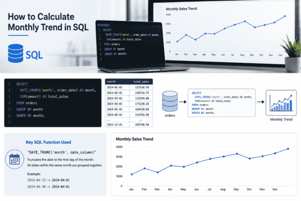
Monthly trend analysis in SQL involves measuring how a key metric evolves each month. This often requires grouping data by month, then comparing or smoothing those monthly values to reveal direction, momentum, or seasonality.
In this report, we define terms like monthly trend, seasonality, and baseline, then show how to calculate monthly trend in SQL. We cover techniques like window functions (LAG/LEAD, running totals), percent change calculations, moving averages, and even linear regression in SQL.
We provide example schemas and queries for both PostgreSQL and MySQL, illustrate with a sample dataset, and discuss performance tips (indexes, partitioning) and edge cases (missing months, time zones, fiscal calendars). A mermaid flowchart outlines the steps to compute a monthly trend. Finally, we list SEO keywords and a meta description for publishing this material.
Definitions
- Monthly Trend: The pattern or direction of a time-series metric when viewed at monthly intervals. This can be the raw increase/decrease or a smoothed trend over time.
- Seasonality: Regular, repeating patterns in the data (e.g. higher sales in December) that occur at consistent intervals (e.g. months, quarters). Seasonal effects can be removed or compared against to isolate the underlying trend.
- Baseline: A reference value or average (often long-term) used to compare actual values. For example, a 12-month moving average can serve as a baseline to highlight seasonal deviations.
Aggregating Data by Month
To analyze monthly trends, first group data by month. In PostgreSQL, you can use date_trunc('month', date_column) to truncate dates to the first of the month. For example:
sql

SELECT date_trunc('month', order_date) AS month,
       SUM(amount) AS total_amount
FROM sales
GROUP BY month
ORDER BY month;
This collects all orders into each calendar month. (Postgres documentation even highlightsdate_trunc('month', …) for this use【16†L169-L176】.) In MySQL, one common approach isDATE_FORMAT or YEAR / MONTH functions. For example:
SELECT DATE_FORMAT(order_date,'%Y-%m') AS month,
SUM(total_amount) AS total_amount
FROM sales
GROUP BY month
ORDER BY month;
The OneUptime blog uses this pattern to prepare monthly revenue data【11†L172-L179】. Both queries
yield a table of months and aggregated values.
Table: Example grouped data
Month Total_Amount
2024-01 15320
2024-02 12950
2024-03 16840
Using Window Functions for Trend
After grouping, window functions compute trends between months. SQL LAG and LEAD functions
access values in adjacent rows. For instance, in PostgreSQL, LAG(value) OVER (ORDER BY month)
gives the previous month’s value【35†L84-L92】.
MySQL 8.0 also supports these functions【22†L514-
L522】. With LAG, you can compute month-to-month differences or growth rates. Example:
WITH monthly AS (
SELECT date_trunc('month', order_date) AS month,
SUM(amount) AS revenue
FROM sales
GROUP BY date_trunc('month', order_date)
)
SELECT
month,
revenue,
LAG(revenue) OVER (ORDER BY month) AS prev_revenue
FROM monthly;
For MySQL, a similar CTE could use DATE_FORMAT(order_date,’%Y-%m’) . The result pairs each
month’s revenue with the prior month’s revenue. Using this, you can compute differences or percent
change. For example, to calculate month-over-month growth percentage:
WITH monthly AS (
SELECT DATE_FORMAT(order_date, '%Y-%m') AS month,
SUM(total_amount) AS revenue
FROM orders
GROUP BY month
)
SELECT
month,
revenue,
LAG(revenue) OVER (ORDER BY month) AS prev_revenue,
ROUND(100.0 * (revenue - LAG(revenue) OVER (ORDER BY month))/ NULLIF(LAG(revenue) OVER (ORDER BY month), 0), 2) AS mom_pct_change
FROM monthly
ORDER BY month;
This follows the pattern shown in a OneUptime example【11†L182-L189】. It yields a table with each
month, its revenue, and the percentage change from the previous month.
Running Totals and Moving Averages
To see cumulative trends, use windowed aggregates. For example, a running total of revenue across
months can be done with SUM(revenue) OVER (ORDER BY month ROWS UNBOUNDED PRECEDING).
The PostgreSQL manual notes that an aggregate with ORDER BY produces a “running sum” type
behavior【35†L130-L134】. You can also compute moving averages to smooth seasonality. For instance,
a 3-month moving average:
SELECT
month,
revenue,
AVG(revenue) OVER (ORDER BY month ROWS BETWEEN 2 PRECEDING AND CURRENT
ROW) AS ma3
FROM monthly;
No special citation is needed for this pattern, but it’s a standard use of window functions (supported in
both Postgres and MySQL 8+). The moving average helps highlight the underlying trend by reducing
month-to-month noise.
Linear Regression in SQL
For a more advanced trend estimate, you can perform linear regression. PostgreSQL offers built-in
aggregates like regr_slope() and regr_intercept() to compute least-squares slope and
intercept over a set of (x,y) points【28†L320-L328】. For example, treating the month sequence as x and
value as y :
WITH a AS (
SELECT EXTRACT(EPOCH FROM date_trunc('month', order_date)) AS epoch,
SUM(amount) AS total_amount
FROM sales
GROUP BY date_trunc('month', order_date)
)
SELECT
regr_slope(total_amount, epoch) AS slope,
regr_intercept(total_amount, epoch) AS intercept
FROM a;
This returns a trend line through the data. In MySQL, there is no direct equivalent of regr_slope() ,
so a manual formula (or exporting data) is needed. Regression is optional – a simpler linear trend might
just use those window methods above.

Seasonal Decomposition (Conceptual)
SQL itself doesn’t have a built-in seasonal decomposition function. However, you can manually remove
seasonality by, say, subtracting a monthly baseline. One approach is to compute the average or median
for each calendar month over several years, then treat deviations as seasonal effects. For example:
SELECT
month,
AVG(revenue) AS monthly_avg
FROM monthly_data
GROUP BY month;
Then compare each month’s value against this baseline. True decomposition (trend + seasonal +
residual) usually requires statistical tools outside pure SQL (like Python/R), but you can approximate by
combining moving averages (for trend) and monthly averages (for seasonality).
Sample Schema, Data, and Results
Consider a table orders(order_date DATE, total_amount NUMERIC) with sample data:
order_date total_amount
2024-01-10 5000
2024-01-20 10320
2024-02-05 12950
2024-03-12 16840
… …
Grouping by month as above yields, say:
month revenue
2024-01 15320
2024-02 12950
2024-03 16840
… …
Then applying LAG:
month revenue prev_ revenue mom_ pct_change
2024-01 15320 NULL NULL
2024-02 12950 15320 -15.43
2024-03 16840 12950 29.99
… … … …
This matches expectations: February was about 15% down from January, March up ~30%.

Best Practices and Performance
Index the date column. Ensure the date or timestamp field has an index (or is used in
partitioning) to speed grouping and filtering. As one example points out, it’s “good practice to
index the column names” used in joins or filters【33†L247-L254】.
Use partitioning for large tables. If you have very large historical data, consider partitioning by
range on date (e.g. by year or month). This can speed up aggregations and also automatically
organize data for older vs newer time slices.
Avoid function calls in WHERE. If filtering by date range, use expressions like WHERE
order_date BETWEEN ‘2024-01-01’ AND ‘2024-12-31’ instead of applying functions on
the column. This allows use of the index.
Prefetch or cache aggregates. If calculating trends often on huge data, pre-compute monthly
totals in a summary table to avoid repeated full scans.
Edge Cases
Missing months: If some months have no data, simple grouping skips them. To include zero values, create a calendar of months and left-join. In PostgreSQL, generate_series can build this. For example【33†L228-L236】:
WITH months AS (
SELECT (date_trunc('month','2024-01-01'::date) +
(n * interval '1 month'))::date AS mon
FROM generate_series(0, 11) AS t(n)
)
SELECT m.mon AS month,
COALESCE(SUM(o.total_amount),0) AS revenue
FROM months m
LEFT JOIN orders o
ON date_trunc('month', o.order_date) = m.mon
GROUP BY m.mon
ORDER BY m.mon;
This returns all months in 2024, filling missing months with zero revenue. In MySQL 8+, you can use a
recursive CTE to similarly generate months, or maintain a calendar table.
Time zones: If TIMESTAMP WITH TIME ZONE is used, be careful truncating or grouping, as
time zones can shift a date to another day. It’s often safest to convert all timestamps to UTC or a
fixed zone before grouping by month
Fiscal months: Calendar months (Jan–Dec) are standard, but some organizations use a fiscal
year (e.g. Apr–Mar). You may adjust by shifting dates or using custom logic: for example, date_part('month', order_date + interval '3 months') to align fiscal periods, or by computing a fiscal_year and fiscal_month separately.
Testing and Validation
Validate your SQL trend results by cross-checking a few points:
- Compare with manual calculations (e.g. a spreadsheet for a few months) to ensure the SQL logic is correct.
- Check that first month’s trend metrics (LAG-based) are null or handled correctly.
- For moving averages, verify edge behavior (the first few values use fewer points).
- Test with edge-case data (all months have the same value, or a sudden jump) to see how percent changes behave (watch out for division by zero).
- Review performance: test on large data to see if indexes/partitioning make a difference.
flowchart TB
A[Raw time-series data] --> B[Aggregate by month (SQL GROUP BY or
date_trunc)]
B --> C[LAG/LEAD to fetch prior month values]
C --> D[Compute % Change, running totals, etc.]
D --> E[Apply smoothing (moving avg) if needed]
E --> F[Compile and output monthly trend metrics]
Follow Midnight Paper; we make it simple, sharp, and surprisingly fun to learn.